Exploring Financial Data with the Nasdaq Data Link API

Introduction

This project explores financial data retrieved from the Nasdaq Data Link API using Python. The analysis focuses on the Accrued Expenses Turnover financial metric and examines how this metric changes over time for different companies.

The main objectives are to retrieve financial data through an API, transform the JSON response into a Pandas DataFrame, clean and filter the dataset, analyze financial trends from 2010 to 2015, compare results across geographical regions, and visualize the findings using Matplotlib.

Code [1]

import requests
import pandas as pd
import matplotlib.pyplot as plt

from google.colab import userdata

api_key = userdata.get('NASDAQ_API_KEY')

print("Libraries imported and API key loaded successfully.")

Output

Libraries imported and API key loaded successfully.

Nasdaq Data Link API

For this project, the financial data is retrieved from the MER/F1 table using the Nasdaq Data Link Tables API.

The API allows parameters to filter rows, select specific columns, and control the number of results returned. For this first request, only 10 rows will be retrieved so that the JSON response can be inspected easily.

Authenticated users have higher API usage limits than anonymous users, so the API key is included with each request.

Code [2]

api_url = "https://data.nasdaq.com/api/v3/datatables/MER/F1.json"

params = {
    "api_key": api_key,
    "qopts.per_page": 10
}

response = requests.get(api_url, params=params)

print("Status code:", response.status_code)

json_data = response.json()

print("Rows returned:", len(json_data["datatable"]["data"]))
print("Columns returned:", len(json_data["datatable"]["columns"]))

print("\nColumn names:")
print([column["name"] for column in json_data["datatable"]["columns"]])

print("\nFirst row:")
print(json_data["datatable"]["data"][0])

Output

Status code: 200
Rows returned: 10
Columns returned: 32

Column names:
['compnumber', 'reportid', 'mapcode', 'amount', 'reportdate', 'reporttype', 'auditorstatus', 'currency', 'consolidated', 'longname', 'shortname', 'status', 'countrycode', 'region', 'cik', 'mic', 'ticker', 'exchange', 'address1', 'address2', 'address3', 'address4', 'city', 'statecode', 'country', 'zipcode', 'phonenumber', 'faxnumber', 'website', 'fye', 'indicator', 'statement']

First row:
[2438, 1868192544, -1802, 10.481948, '2011-06-30', 'Q2', 'U', 'EUR', 'True', 'Deutsche Bank AG', 'Deutsche Bank AG', 'Active', 'DEU', 'Europe', 1159508, '5.1.1', 'DB', 'NYS', 'Taunusanlage 12', None, None, None, 'Frankfurt am Main', None, 'DEU', '60325', '(49) 69 910 00', '(49) 69 910 34 225', 'www.db.com', '2025-12-31', 'Accrued Expenses Turnover', 'Derived']

Processing the JSON Data

The API response contains the financial data inside the data section and the corresponding column information inside the columns section.

To make the dataset easier to analyze, the JSON response will be converted into a Pandas DataFrame.

Code [3]

params["qopts.per_page"] = 10000

response = requests.get(api_url, params=params)
json_data = response.json()

data = json_data["datatable"]["data"]

columns = [
    column["name"]
    for column in json_data["datatable"]["columns"]
]

df_metric = pd.DataFrame(data, columns=columns)

df_metric.head()

Output

	compnumber	reportid	mapcode	amount	reportdate	reporttype	auditorstatus	currency	consolidated	longname	...	city	statecode	country	zipcode	phonenumber	faxnumber	website	fye	indicator	statement
0	2438	1868192544	-1802	10.481948	2011-06-30	Q2	U	EUR	True	Deutsche Bank AG	...	Frankfurt am Main	None	DEU	60325	(49) 69 910 00	(49) 69 910 34 225	www.db.com	2025-12-31	Accrued Expenses Turnover	Derived
1	2438	1868216112	-1802	8.161754	2011-09-30	Q3	U	EUR	True	Deutsche Bank AG	...	Frankfurt am Main	None	DEU	60325	(49) 69 910 00	(49) 69 910 34 225	www.db.com	2025-12-31	Accrued Expenses Turnover	Derived
2	2438	1885063456	-1802	10.788213	2012-06-30	Q2	U	EUR	True	Deutsche Bank AG	...	Frankfurt am Main	None	DEU	60325	(49) 69 910 00	(49) 69 910 34 225	www.db.com	2025-12-31	Accrued Expenses Turnover	Derived
3	2438	1885087024	-1802	9.437545	2012-09-30	Q3	U	EUR	True	Deutsche Bank AG	...	Frankfurt am Main	None	DEU	60325	(49) 69 910 00	(49) 69 910 34 225	www.db.com	2025-12-31	Accrued Expenses Turnover	Derived
4	2438	1901934112	-1802	8.755041	2013-06-30	Q2	U	EUR	True	Deutsche Bank AG	...	Frankfurt am Main	None	DEU	60325	(49) 69 910 00	(49) 69 910 34 225	www.db.com	2025-12-31	Accrued Expenses Turnover	Derived

5 rows × 32 columns

Understanding the Dataset

Before starting the analysis, it is useful to inspect the structure of the DataFrame and identify the columns that are relevant for the project.

The main columns needed are:

indicator: identifies the financial metric.
country: identifies the country of the company.
longname: contains the company name.
reportdate: contains the reporting date.
reporttype: identifies the type of financial report.
amount: contains the value of the financial metric.

These columns are important because they allow us to compare companies, analyze changes over time, and compare results between countries.

Code [4]

print("DataFrame shape:", df_metric.shape)

df_metric.info()

Output

DataFrame shape: (10000, 32)
<class 'pandas.core.frame.DataFrame'>
RangeIndex: 10000 entries, 0 to 9999
Data columns (total 32 columns):
 #   Column         Non-Null Count  Dtype  
---  ------         --------------  -----  
 0   compnumber     10000 non-null  int64  
 1   reportid       10000 non-null  int64  
 2   mapcode        10000 non-null  int64  
 3   amount         10000 non-null  float64
 4   reportdate     10000 non-null  object 
 5   reporttype     10000 non-null  object 
 6   auditorstatus  9999 non-null   object 
 7   currency       10000 non-null  object 
 8   consolidated   10000 non-null  object 
 9   longname       10000 non-null  object 
 10  shortname      10000 non-null  object 
 11  status         10000 non-null  object 
 12  countrycode    10000 non-null  object 
 13  region         10000 non-null  object 
 14  cik            10000 non-null  int64  
 15  mic            10000 non-null  object 
 16  ticker         9380 non-null   object 
 17  exchange       10000 non-null  object 
 18  address1       10000 non-null  object 
 19  address2       6001 non-null   object 
 20  address3       1298 non-null   object 
 21  address4       0 non-null      object 
 22  city           8432 non-null   object 
 23  statecode      5813 non-null   object 
 24  country        10000 non-null  object 
 25  zipcode        9068 non-null   object 
 26  phonenumber    10000 non-null  object 
 27  faxnumber      3681 non-null   object 
 28  website        10000 non-null  object 
 29  fye            10000 non-null  object 
 30  indicator      10000 non-null  object 
 31  statement      10000 non-null  object 
dtypes: float64(1), int64(4), object(27)
memory usage: 2.4+ MB

Code [5]

necessary_columns = [
    "indicator",
    "country",
    "longname",
    "reportdate",
    "reporttype",
    "amount"
]

necessary_columns

Output

['indicator', 'country', 'longname', 'reportdate', 'reporttype', 'amount']

Filtering the Data

The dataset contains many different financial indicators. Since this project focuses on Accrued Expenses Turnover, the DataFrame will be filtered to keep only the relevant columns and rows for this specific metric.

Code [6]

filtered_df = df_metric[necessary_columns].copy()

filtered_df = filtered_df[
    filtered_df["indicator"] == "Accrued Expenses Turnover"
]

filtered_df.head()

Output

	indicator	country	longname	reportdate	reporttype	amount
0	Accrued Expenses Turnover	DEU	Deutsche Bank AG	2011-06-30	Q2	10.481948
1	Accrued Expenses Turnover	DEU	Deutsche Bank AG	2011-09-30	Q3	8.161754
2	Accrued Expenses Turnover	DEU	Deutsche Bank AG	2012-06-30	Q2	10.788213
3	Accrued Expenses Turnover	DEU	Deutsche Bank AG	2012-09-30	Q3	9.437545
4	Accrued Expenses Turnover	DEU	Deutsche Bank AG	2013-06-30	Q2	8.755041

Code [7]

filtered_df["amount"].describe()

Output

	amount
count	139.000000
mean	26.908762
std	33.097291
min	4.689773
25%	9.675670
50%	13.753753
75%	31.777614
max	229.810427

dtype: float64

Statistical Observation

The average Accrued Expenses Turnover is approximately 26.91, while the median is around 13.75. The values range from 4.69 to 229.81, with a standard deviation of approximately 33.10.

The large difference between the median and the maximum value suggests that some companies have much higher turnover values than others. This explains the relatively high variability in the dataset.

Enhancing the DataFrame

To make the dataset easier to read, the country codes will be converted into full country names. The longname column will also be renamed to company_name, and the column names will use a consistent naming style.

Code [8]

country_mapping = {
    "USA": "United States of America",
    "DEU": "Germany",
    "JPN": "Japan",
    "CYM": "Cayman Islands",
    "BHS": "Bahamas",
    "IRL": "Ireland",
    "GBR": "United Kingdom"
}

def get_country_name(country):
    return country_mapping.get(country, country)

Code [9]

updated_df = filtered_df.copy()

updated_df["country_name"] = updated_df["country"].apply(get_country_name)

updated_df = updated_df.rename(columns={
    "longname": "company_name",
    "reportdate": "report_date",
    "reporttype": "report_type"
})

updated_df.head()

Output

	indicator	country	company_name	report_date	report_type	amount	country_name
0	Accrued Expenses Turnover	DEU	Deutsche Bank AG	2011-06-30	Q2	10.481948	Germany
1	Accrued Expenses Turnover	DEU	Deutsche Bank AG	2011-09-30	Q3	8.161754	Germany
2	Accrued Expenses Turnover	DEU	Deutsche Bank AG	2012-06-30	Q2	10.788213	Germany
3	Accrued Expenses Turnover	DEU	Deutsche Bank AG	2012-09-30	Q3	9.437545	Germany
4	Accrued Expenses Turnover	DEU	Deutsche Bank AG	2013-06-30	Q2	8.755041	Germany

Code [10]

updated_df["country_name"].value_counts()

Output

	count
country_name
United States of America	31
Japan	27
Cayman Islands	27
Ireland	25
Bahamas	19
Germany	6
United Kingdom	4

dtype: int64

Financial Trends Over Time

To analyze how Accrued Expenses Turnover changes over time, the data will be restricted to the period from 2010 to 2015.

The analysis will focus on the company name, report date, and financial amount.

Code [11]

updated_df["report_date"] = pd.to_datetime(updated_df["report_date"])

updated_df = updated_df[
    (updated_df["report_date"].dt.year >= 2010) &
    (updated_df["report_date"].dt.year <= 2015)
]

updated_df.head()

Output

	indicator	country	company_name	report_date	report_type	amount	country_name
0	Accrued Expenses Turnover	DEU	Deutsche Bank AG	2011-06-30	Q2	10.481948	Germany
1	Accrued Expenses Turnover	DEU	Deutsche Bank AG	2011-09-30	Q3	8.161754	Germany
2	Accrued Expenses Turnover	DEU	Deutsche Bank AG	2012-06-30	Q2	10.788213	Germany
3	Accrued Expenses Turnover	DEU	Deutsche Bank AG	2012-09-30	Q3	9.437545	Germany
4	Accrued Expenses Turnover	DEU	Deutsche Bank AG	2013-06-30	Q2	8.755041	Germany

Code [12]

relevant_data = updated_df[
    ["company_name", "report_date", "amount"]
].copy()

relevant_data.head()

Output

	company_name	report_date	amount
0	Deutsche Bank AG	2011-06-30	10.481948
1	Deutsche Bank AG	2011-09-30	8.161754
2	Deutsche Bank AG	2012-06-30	10.788213
3	Deutsche Bank AG	2012-09-30	9.437545
4	Deutsche Bank AG	2013-06-30	8.755041

Code [13]

plt.figure(figsize=(12, 6))

for company in relevant_data["company_name"].unique():
    company_data = relevant_data[
        relevant_data["company_name"] == company
    ].sort_values("report_date")

    plt.plot(
        company_data["report_date"],
        company_data["amount"],
        label=company
    )

plt.title("Accrued Expenses Turnover by Company (2010–2015)")
plt.xlabel("Report Date")
plt.ylabel("Accrued Expenses Turnover")

plt.legend(
    title="Company",
    bbox_to_anchor=(1.05, 1),
    loc="upper left"
)

plt.tight_layout()
plt.show()

Output

Trend Observation

The chart shows that Accrued Expenses Turnover varies considerably between companies during the 2010–2015 period.

Some companies show relatively stable values, while others have larger increases or decreases over time. This suggests that companies manage their accrued expenses differently.

Geographical Region Analysis

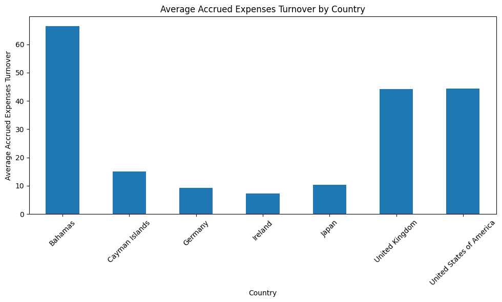
The data can also be grouped by country to compare the average Accrued Expenses Turnover across different geographical regions.

For this analysis, the average amount will be calculated for each country.

Code [14]

country_avg = updated_df.groupby("country_name")["amount"].mean()

country_avg

Output

	amount
country_name
Bahamas	66.515369
Cayman Islands	15.060796
Germany	9.288999
Ireland	7.264400
Japan	10.376605
United Kingdom	44.166750
United States of America	44.377585

dtype: float64

Code [15]

plt.figure(figsize=(10, 6))

country_avg.plot(kind="bar")

plt.title("Average Accrued Expenses Turnover by Country")
plt.xlabel("Country")
plt.ylabel("Average Accrued Expenses Turnover")

plt.xticks(rotation=45)
plt.tight_layout()
plt.show()

Output

Code [16]

country_avg

Output

	amount
country_name
Bahamas	66.515369
Cayman Islands	15.060796
Germany	9.288999
Ireland	7.264400
Japan	10.376605
United Kingdom	44.166750
United States of America	44.377585

dtype: float64

Conclusion

In this project, financial data was retrieved from the Nasdaq Data Link API and converted into a Pandas DataFrame for analysis.

The analysis focused on Accrued Expenses Turnover. The data showed considerable differences between companies and countries. During the 2010–2015 period, some companies had relatively stable values, while others showed larger changes over time.

When comparing countries, the Bahamas had the highest average Accrued Expenses Turnover in this dataset, at approximately 66.52. The United States and the United Kingdom also had relatively high averages, at approximately 44.38 and 44.17 respectively.

These results show how Python, Pandas, and Matplotlib can be used together to retrieve, clean, analyze, and visualize financial data from an API.

Nasdaq Financial Data Analysis

Project library

Exploring Financial Data with the Nasdaq Data Link API

Introduction

Nasdaq Data Link API

Processing the JSON Data

Understanding the Dataset

Filtering the Data

Statistical Observation

Enhancing the DataFrame

Financial Trends Over Time

Trend Observation

Geographical Region Analysis

Conclusion

Project report