Cultural Differences in Finance
Survey analysis of honesty, ethical judgments and cultural differences, using five regression models with robust standard errors and a Europe–Asia comparison.
Project library
Read the original notebook, including its code, tables and saved charts. No account is required.
Data preparation
Load the survey, select valid responses, and combine Hong Kong with China. Define honesty importance and the outcome C_minus_B = E33 - E32, where higher values mean a more favorable evaluation of the reporter relative to the student permitting copying. All regressions use HC3 robust standard errors.
from pathlib import Path

import numpy as np
import pandas as pd
import pyreadstat
import statsmodels.formula.api as smf
import matplotlib.pyplot as plt
from IPython.display import display

sav_path = Path.cwd() / "data_combined_20.08.2026.sav"
columns = ["imp3", "E31", "E32", "E33", "cntry", "age", "gender", "degree", "PDI1", "IDV"]
df, meta = pyreadstat.read_sav(
    str(sav_path), usecols=columns, apply_value_formats=False, user_missing=True
)

valid = (
    df[["imp3", "E31", "E32", "E33"]].isin([1, 2, 3, 4, 5]).all(axis=1)
    & df["age"].between(16, 100)
    & df["cntry"].isin(range(1, 10))
    & df["gender"].isin([1, 2, 3])
    & df["degree"].isin([1, 2, 3, 4, 5])
)
analysis = df.loc[valid].copy()
# Pool Hong Kong with China in the analysis; retain original codes in df.
analysis["cntry"] = analysis["cntry"].replace({7: 4})
country_labels = meta.variable_value_labels["cntry"].copy()
country_labels[4] = "China (incl. Hong Kong)"
country_labels.pop(7, None)
analysis["honesty_importance"] = analysis["imp3"]
analysis["C_minus_B"] = analysis["E33"] - analysis["E32"]
analysis["region"] = np.where(analysis["cntry"].isin([1, 2, 9]), "Western", "Eastern")
for variable in ["cntry", "gender", "degree"]:
    analysis[variable] = analysis[variable].astype(int).astype("category")

print(f"Common regression sample: {len(analysis):,} of {len(df):,} rows "
f"({len(df) - len(analysis):,} excluded by validity / complete-case rules).")Common regression sample: 2,734 of 7,194 rows (4,460 excluded by validity / complete-case rules).
Regression tables and plots
Define a shared format for coefficient tables, significance marks, confidence intervals, and plots. Points show respondents, while the fitted line shows adjusted model predictions.
# Shared presentation; each regression is fitted in its own cell below.
def show_regression(result, title, sample=None, predictors=None, country_lines=False):
    if sample is None:
        sample = analysis
    if predictors is None:
        predictors = ["honesty_importance"]

    ci = result.conf_int()
    table = pd.DataFrame({
        "beta": result.params,
        "HC3 SE": result.bse,
        "p-value": result.pvalues,
        "95% CI lower": ci[0],
        "95% CI upper": ci[1],
    })
    table["significance"] = pd.cut(
        table["p-value"], bins=[-np.inf, .001, .01, .05, .10, np.inf],
        labels=["***", "**", "*", ".", ""], right=False
    )
    table = table.rename(index={
        "PDI1": "Power distance (PDI1)", "IDV": "Individualism (IDV)"
    })
    print(title)
    print(f"N = {int(result.nobs):,} | R² = {result.rsquared:.3f} | "
          f"Adjusted R² = {result.rsquared_adj:.3f} | Standard errors: {result.cov_type}")
    display(table.style.format({
        "beta": "{:.4f}", "HC3 SE": "{:.4f}", "p-value": "{:.3g}",
        "95% CI lower": "{:.4f}", "95% CI upper": "{:.4f}"
    }))

    for predictor in predictors:
        if predictor == "honesty_importance":
            levels = np.arange(1, 6)
            ticks = levels
            xlabel = "Honesty importance (1 = least, 5 = very important)"
            xlim = (.7, 5.3)
            jitter_width = .12
        else:
            # Limit the fitted line to the observed score range.
            levels = np.linspace(sample[predictor].min(), sample[predictor].max(), 40)
            ticks = [1, 2, 3, 4]
            xlabel = "Rejection of dishonesty (ten-item mean; 4 = strongest rejection of dishonesty)"
            xlim = (.8, 4.2)
            jitter_width = .025

        rng = np.random.default_rng(42)
        plot_x = sample[predictor].to_numpy() + rng.uniform(-jitter_width, jitter_width, len(sample))
        plot_y = sample["C_minus_B"].to_numpy() + rng.uniform(-.10, .10, len(sample))
        fig, ax = plt.subplots(figsize=(8, 5))
        for region, color in [("Western", "blue"), ("Eastern", "red")]:
            mask = sample["region"].eq(region).to_numpy()
            ax.scatter(plot_x[mask], plot_y[mask], color=color, s=13, alpha=.18,
                       edgecolors="none", label=region)
        mean_predictions = [
            result.predict(sample.assign(**{predictor: level})).mean()
            for level in levels
        ]
        ax.plot(levels, mean_predictions, color="black", linewidth=2.5,
                label="Model mean prediction", zorder=3)
        if country_lines and predictor == "honest_behavior":
            line_styles = ["-", "--", "-.", ":", (0, (5, 1)), (0, (3, 1, 1, 1))]
            for i, country in enumerate(sample["cntry"].cat.categories):
                country_sample = sample.loc[sample["cntry"].eq(country)]
                if country_sample.empty:
                    continue
                country_levels = np.linspace(
                    country_sample[predictor].min(), country_sample[predictor].max(), 30
                )
                predictions = [
                    result.predict(country_sample.assign(**{predictor: level})).mean()
                    for level in country_levels
                ]
                color = "blue" if country in [1, 2, 9] else "red"
                ax.plot(country_levels, predictions, color=color,
                        linestyle=line_styles[i % len(line_styles)], linewidth=1.8,
                        label=country_labels[country])
        ax.axhline(0, color="gray", linestyle="--", linewidth=1)
        ax.set(xlabel=xlabel,
               ylabel="C_minus_B (reporter − student permitting copying)",
               title=title, xticks=ticks, yticks=range(-4, 5),
               xlim=xlim, ylim=(-4.3, 4.3))
        if country_lines and predictor == "honest_behavior":
            ax.legend(bbox_to_anchor=(1.02, 1), loc="upper left", fontsize=8)
        else:
            ax.legend()
        fig.tight_layout()
        plt.show()
        plt.close(fig)
Model 1: honesty importance
Estimate the association between honesty importance and relative evaluation of the reporter.
model_1 = smf.ols(
    "C_minus_B ~ honesty_importance", data=analysis, missing="raise"
).fit(cov_type="HC3")
show_regression(model_1, "Model 1: honesty importance")Model 1: honesty importance N = 2,734 | R² = 0.000 | Adjusted R² = -0.000 | Standard errors: HC3
| beta | HC3 SE | p-value | 95% CI lower | 95% CI upper | significance | |
|---|---|---|---|---|---|---|
| Intercept | 0.1428 | 0.1169 | 0.222 | -0.0864 | 0.3720 | |
| honesty_importance | -0.0224 | 0.0286 | 0.433 | -0.0784 | 0.0336 |

Model 2: country controls
Add country fixed effects to account for differences in evaluation levels across countries.
model_2 = smf.ols(
    "C_minus_B ~ honesty_importance + C(cntry)", data=analysis, missing="raise"
).fit(cov_type="HC3")
show_regression(model_2, "Model 2: honesty importance + country fixed effects")Model 2: honesty importance + country fixed effects N = 2,734 | R² = 0.211 | Adjusted R² = 0.209 | Standard errors: HC3
| beta | HC3 SE | p-value | 95% CI lower | 95% CI upper | significance | |
|---|---|---|---|---|---|---|
| Intercept | -1.6152 | 0.1411 | 2.36e-30 | -1.8917 | -1.3387 | *** |
| C(cntry)[T.2] | 0.2044 | 0.2112 | 0.333 | -0.2096 | 0.6184 | |
| C(cntry)[T.3] | 2.0064 | 0.0878 | 1.89e-115 | 1.8342 | 2.1786 | *** |
| C(cntry)[T.4] | 1.7687 | 0.0940 | 4.76e-79 | 1.5846 | 1.9529 | *** |
| C(cntry)[T.5] | 1.7675 | 0.0937 | 2.53e-79 | 1.5838 | 1.9512 | *** |
| C(cntry)[T.6] | 2.4065 | 0.1739 | 1.52e-43 | 2.0656 | 2.7473 | *** |
| C(cntry)[T.8] | 1.8178 | 0.1607 | 1.14e-29 | 1.5029 | 2.1328 | *** |
| honesty_importance | 0.0670 | 0.0295 | 0.0232 | 0.0092 | 0.1248 | * |

Model 3: demographic controls
Add age, gender, and education to the honesty-importance and country model.
model_3 = smf.ols(
    "C_minus_B ~ honesty_importance + C(cntry) + age + C(gender) + C(degree)",
    data=analysis, missing="raise"
).fit(cov_type="HC3")
show_regression(model_3, "Model 3: country fixed effects + demographic controls")Model 3: country fixed effects + demographic controls N = 2,734 | R² = 0.218 | Adjusted R² = 0.214 | Standard errors: HC3
| beta | HC3 SE | p-value | 95% CI lower | 95% CI upper | significance | |
|---|---|---|---|---|---|---|
| Intercept | -2.0075 | 0.1989 | 5.97e-24 | -2.3974 | -1.6176 | *** |
| C(cntry)[T.2] | 0.2417 | 0.2091 | 0.248 | -0.1682 | 0.6516 | |
| C(cntry)[T.3] | 1.9419 | 0.0973 | 1.4e-88 | 1.7512 | 2.1327 | *** |
| C(cntry)[T.4] | 1.7591 | 0.1006 | 2.04e-68 | 1.5619 | 1.9564 | *** |
| C(cntry)[T.5] | 1.7962 | 0.0951 | 1.54e-79 | 1.6098 | 1.9826 | *** |
| C(cntry)[T.6] | 2.4513 | 0.1772 | 1.53e-43 | 2.1041 | 2.7985 | *** |
| C(cntry)[T.8] | 1.8336 | 0.1629 | 2.14e-29 | 1.5143 | 2.1528 | *** |
| C(gender)[T.2] | 0.1051 | 0.0641 | 0.101 | -0.0205 | 0.2306 | |
| C(gender)[T.3] | 0.3881 | 0.4976 | 0.435 | -0.5872 | 1.3635 | |
| C(degree)[T.2] | 0.0748 | 0.0767 | 0.329 | -0.0755 | 0.2251 | |
| C(degree)[T.3] | 0.2847 | 0.1110 | 0.0103 | 0.0671 | 0.5024 | * |
| C(degree)[T.4] | -0.1559 | 0.2805 | 0.578 | -0.7057 | 0.3939 | |
| C(degree)[T.5] | -0.0867 | 0.1814 | 0.633 | -0.4422 | 0.2688 | |
| honesty_importance | 0.0645 | 0.0293 | 0.0277 | 0.0071 | 0.1219 | * |
| age | 0.0113 | 0.0057 | 0.0483 | 0.0001 | 0.0225 | * |

Rejection of dishonesty: ten survey items
Use all ten E5 questions, including E52 and E510, to measure rejection of dishonest actions.
Response distributions and Cronbach’s alpha
Show response counts and percentages, then calculate Cronbach’s alpha to assess internal consistency. Keep responses from 1 to 4, treat other responses as missing, and require valid answers to all ten questions.
e5_items = [f"E5{i}" for i in range(1, 11)]
e5_raw, e5_meta = pyreadstat.read_sav(
    str(sav_path), usecols=e5_items, apply_value_formats=False, user_missing=True
)
# Row indices refer to the same source file loaded above.
e5_sample = e5_raw.loc[analysis.index].copy()
item_names = {
    "E51": "Buying stolen goods",
    "E52": "Keeping money found in the street",
    "E53": "Having an affair while married",
    "E54": "Not reporting damage to a parked vehicle",
    "E55": "Fare evasion",
    "E56": "Tax cheating",
    "E57": "Accepting a bribe",
    "E58": "Fabricating a job application",
    "E59": "Promising a child a reward that will not be given",
    "E510": "Lying about a dangerous wolf to keep a child out of the forest",
}
response_labels = {
    1: "1 Always justified", 2: "2 Sometimes justified",
    3: "3 Rarely justified", 4: "4 Never justified", 5: "5 Don't know"
}

response_counts = pd.DataFrame({
    label: e5_sample.eq(value).sum() for value, label in response_labels.items()
})
response_counts["Missing"] = e5_sample.isna().sum()
response_counts["Invalid code"] = (
    e5_sample.notna() & ~e5_sample.isin([1, 2, 3, 4, 5])
).sum()
response_percent = 100 * response_counts / len(e5_sample)
response_table = response_counts.copy().astype(str)
for column in response_counts:
    response_table[column] = [
        f"{count:,} ({percent:.1f}%)"
        for count, percent in zip(response_counts[column], response_percent[column])
    ]
response_table.insert(0, "Question", pd.Series(item_names))
response_table.index.name = "Item"
print(f"Response table denominator: {len(e5_sample):,} regression-sample respondents per row.")
with pd.option_context("display.max_columns", None, "display.max_colwidth", None):
    display(response_table)

# Raw Cronbach's alpha: k/(k-1) * (1 - sum(item variances)/variance(total)).
e5_valid = e5_sample.where(e5_sample.isin([1, 2, 3, 4]))
e5_complete = e5_valid.dropna()
k = len(e5_items)
if len(e5_complete) < 2:
    raise ValueError("Too few complete respondents to estimate Cronbach's alpha.")
item_variances = e5_complete.var(ddof=1)
total_variance = e5_complete.sum(axis=1).var(ddof=1)
if total_variance <= 0:
    raise ValueError("Cronbach's alpha is undefined: total scores have no variance.")
cronbach_alpha = k / (k - 1) * (1 - item_variances.sum() / total_variance)
alpha_summary = pd.DataFrame({
    "Items": [k],
    "Starting sample N": [len(e5_sample)],
    "Complete ten-item N": [len(e5_complete)],
    "Excluded for missing / don't know / invalid": [len(e5_sample) - len(e5_complete)],
    "Cronbach's alpha": [cronbach_alpha],
})
display(alpha_summary.style.format({"Cronbach's alpha": "{:.3f}"}))
print(f"Cronbach's alpha = {cronbach_alpha:.3f}; N = {len(e5_complete):,} complete respondents.")Response table denominator: 2,734 regression-sample respondents per row.
| Question | 1 Always justified | 2 Sometimes justified | 3 Rarely justified | 4 Never justified | 5 Don't know | Missing | Invalid code | |
|---|---|---|---|---|---|---|---|---|
| Item | ||||||||
| E51 | Buying stolen goods | 43 (1.6%) | 448 (16.4%) | 740 (27.1%) | 1,454 (53.2%) | 47 (1.7%) | 2 (0.1%) | 0 (0.0%) |
| E52 | Keeping money found in the street | 185 (6.8%) | 1,032 (37.7%) | 747 (27.3%) | 721 (26.4%) | 41 (1.5%) | 8 (0.3%) | 0 (0.0%) |
| E53 | Having an affair while married | 37 (1.4%) | 248 (9.1%) | 540 (19.8%) | 1,829 (66.9%) | 76 (2.8%) | 4 (0.1%) | 0 (0.0%) |
| E54 | Not reporting damage to a parked vehicle | 57 (2.1%) | 328 (12.0%) | 857 (31.3%) | 1,438 (52.6%) | 45 (1.6%) | 8 (0.3%) | 1 (0.0%) |
| E55 | Fare evasion | 86 (3.1%) | 514 (18.8%) | 761 (27.8%) | 1,331 (48.7%) | 36 (1.3%) | 5 (0.2%) | 1 (0.0%) |
| E56 | Tax cheating | 79 (2.9%) | 324 (11.9%) | 627 (22.9%) | 1,637 (59.9%) | 57 (2.1%) | 8 (0.3%) | 2 (0.1%) |
| E57 | Accepting a bribe | 30 (1.1%) | 199 (7.3%) | 483 (17.7%) | 1,972 (72.1%) | 47 (1.7%) | 3 (0.1%) | 0 (0.0%) |
| E58 | Fabricating a job application | 57 (2.1%) | 515 (18.8%) | 778 (28.5%) | 1,333 (48.8%) | 44 (1.6%) | 6 (0.2%) | 1 (0.0%) |
| E59 | Promising a child a reward that will not be given | 54 (2.0%) | 472 (17.3%) | 797 (29.2%) | 1,365 (49.9%) | 44 (1.6%) | 2 (0.1%) | 0 (0.0%) |
| E510 | Lying about a dangerous wolf to keep a child out of the forest | 257 (9.4%) | 1,157 (42.3%) | 632 (23.1%) | 639 (23.4%) | 47 (1.7%) | 2 (0.1%) | 0 (0.0%) |
| Items | Starting sample N | Complete ten-item N | Excluded for missing / don't know / invalid | Cronbach's alpha | |
|---|---|---|---|---|---|
| 0 | 10 | 2734 | 2390 | 344 | 0.719 |
Cronbach's alpha = 0.719; N = 2,390 complete respondents.
Model 4: rejection of dishonesty
Average all ten items to create honest_behavior, where higher scores indicate stronger rejection of dishonest actions. Add this score to Model 3 using respondents with complete answers to all ten items.
analysis_4 = analysis.loc[e5_complete.index].copy()
analysis_4["honest_behavior"] = e5_complete.mean(axis=1)
print(f"Model 4 sample: {len(analysis_4):,}; "
      f"{len(analysis) - len(analysis_4):,} fewer respondents than Model 3.")

model_4 = smf.ols(
    "C_minus_B ~ honesty_importance + honest_behavior + C(cntry) + age + C(gender) + C(degree)",
    data=analysis_4, missing="raise"
).fit(cov_type="HC3")
show_regression(
    model_4, "Model 4: both honesty measures + country and demographic controls",
    sample=analysis_4, predictors=["honesty_importance", "honest_behavior"]
)Model 4 sample: 2,390; 344 fewer respondents than Model 3. Model 4: both honesty measures + country and demographic controls N = 2,390 | R² = 0.249 | Adjusted R² = 0.244 | Standard errors: HC3
| beta | HC3 SE | p-value | 95% CI lower | 95% CI upper | significance | |
|---|---|---|---|---|---|---|
| Intercept | -3.8916 | 0.3255 | 6.05e-33 | -4.5296 | -3.2537 | *** |
| C(cntry)[T.2] | 0.5510 | 0.2146 | 0.0102 | 0.1304 | 0.9717 | * |
| C(cntry)[T.3] | 1.8799 | 0.1027 | 6.54e-75 | 1.6787 | 2.0811 | *** |
| C(cntry)[T.4] | 1.6785 | 0.1077 | 8.54e-55 | 1.4674 | 1.8895 | *** |
| C(cntry)[T.5] | 1.8086 | 0.1029 | 4.13e-69 | 1.6069 | 2.0103 | *** |
| C(cntry)[T.6] | 2.4258 | 0.1844 | 1.52e-39 | 2.0645 | 2.7871 | *** |
| C(cntry)[T.8] | 1.7472 | 0.1839 | 2.07e-21 | 1.3868 | 2.1077 | *** |
| C(gender)[T.2] | 0.1050 | 0.0674 | 0.119 | -0.0271 | 0.2371 | |
| C(gender)[T.3] | 0.6081 | 0.6350 | 0.338 | -0.6365 | 1.8528 | |
| C(degree)[T.2] | 0.0934 | 0.0825 | 0.258 | -0.0684 | 0.2552 | |
| C(degree)[T.3] | 0.3335 | 0.1184 | 0.00484 | 0.1015 | 0.5655 | ** |
| C(degree)[T.4] | -0.0536 | 0.2816 | 0.849 | -0.6055 | 0.4984 | |
| C(degree)[T.5] | -0.0870 | 0.1969 | 0.659 | -0.4729 | 0.2990 | |
| honesty_importance | 0.0267 | 0.0303 | 0.379 | -0.0327 | 0.0861 | |
| honest_behavior | 0.6642 | 0.0845 | 3.84e-15 | 0.4986 | 0.8298 | *** |
| age | 0.0060 | 0.0063 | 0.345 | -0.0064 | 0.0183 |


Model 5: power distance and individualism
Add the existing power-distance index PDI1 and individualism index IDV to Model 4. Retain their original units and use respondents with both indices available.
# Retain the existing index units; require both additional controls for Model 5 only.
analysis_5 = analysis_4.loc[
    np.isfinite(analysis_4[["PDI1", "IDV"]]).all(axis=1)
].copy()
for variable in ["cntry", "gender", "degree"]:
    analysis_5[variable] = analysis_5[variable].cat.remove_unused_categories()

print(f"Model 5 sample: {len(analysis_5):,}; "
      f"{len(analysis_4) - len(analysis_5):,} fewer respondents than Model 4.")
absent_countries = sorted(set(analysis_4["cntry"]) - set(analysis_5["cntry"]))
print("Countries lost relative to Model 4:",
      [country_labels[code] for code in absent_countries] or "None")

model_5 = smf.ols(
    "C_minus_B ~ honesty_importance + honest_behavior + C(cntry) "
    "+ age + C(gender) + C(degree) + PDI1 + IDV",
    data=analysis_5, missing="raise"
).fit(cov_type="HC3")

show_regression(
    model_5, "Model 5: add power distance and individualism",
    sample=analysis_5, predictors=["honesty_importance", "honest_behavior"]
)Model 5 sample: 2,217; 173 fewer respondents than Model 4. Countries lost relative to Model 4: ['India'] Model 5: add power distance and individualism N = 2,217 | R² = 0.273 | Adjusted R² = 0.267 | Standard errors: HC3
| beta | HC3 SE | p-value | 95% CI lower | 95% CI upper | significance | |
|---|---|---|---|---|---|---|
| Intercept | -3.7999 | 0.3489 | 1.28e-27 | -4.4838 | -3.1160 | *** |
| C(cntry)[T.2] | 0.5511 | 0.2091 | 0.00842 | 0.1411 | 0.9610 | ** |
| C(cntry)[T.3] | 1.7765 | 0.1074 | 1.69e-61 | 1.5661 | 1.9869 | *** |
| C(cntry)[T.4] | 1.6079 | 0.1111 | 1.68e-47 | 1.3903 | 1.8256 | *** |
| C(cntry)[T.5] | 1.8277 | 0.1022 | 1.61e-71 | 1.6274 | 2.0280 | *** |
| C(cntry)[T.6] | 2.3411 | 0.1884 | 1.89e-35 | 1.9719 | 2.7104 | *** |
| C(gender)[T.2] | 0.0696 | 0.0696 | 0.317 | -0.0668 | 0.2059 | |
| C(gender)[T.3] | 0.5522 | 0.6196 | 0.373 | -0.6623 | 1.7666 | |
| C(degree)[T.2] | 0.1057 | 0.0841 | 0.209 | -0.0591 | 0.2705 | |
| C(degree)[T.3] | 0.3990 | 0.1211 | 0.000988 | 0.1616 | 0.6365 | *** |
| C(degree)[T.4] | -0.1221 | 0.2974 | 0.681 | -0.7049 | 0.4607 | |
| C(degree)[T.5] | -0.0364 | 0.1953 | 0.852 | -0.4192 | 0.3464 | |
| honesty_importance | 0.0418 | 0.0311 | 0.179 | -0.0192 | 0.1027 | |
| honest_behavior | 0.6939 | 0.0885 | 4.48e-15 | 0.5205 | 0.8674 | *** |
| age | 0.0077 | 0.0064 | 0.232 | -0.0049 | 0.0202 | |
| Power distance (PDI1) | 0.0005 | 0.0008 | 0.498 | -0.0010 | 0.0021 | |
| Individualism (IDV) | -0.0030 | 0.0008 | 0.000181 | -0.0045 | -0.0014 | *** |


Models 1–5: coefficient comparison
Compare all five models side by side using readable variable names, significance marks, and HC3 standard errors. Include sample sizes and model fit statistics; Models 4 and 5 can use fewer respondents because of their additional data requirements.
import re

comparison_models = {
    "Model 1": model_1, "Model 2": model_2,
    "Model 3": model_3, "Model 4": model_4,
    "Model 5": model_5,
}


def significance_mark(p):
    if p < .001:
        return "***"
    if p < .01:
        return "**"
    if p < .05:
        return "*"
    if p < .10:
        return "·"
    return ""


def readable_term(term):
    names = {
        "Intercept": "Intercept",
        "honesty_importance": "Honesty importance",
        "honest_behavior": "Rejection of dishonesty",
        "age": "Age (years)",
        "PDI1": "Power distance (PDI1)",
        "IDV": "Individualism (IDV)",
    }
    if term in names:
        return names[term]
    match = re.fullmatch(r"C\((cntry|gender|degree)\)\[T\.(\d+)\]", term)
    if match:
        variable, code = match.groups()
        labels = country_labels if variable == "cntry" else meta.variable_value_labels[variable]
        label = labels[int(code)]
        prefix = {"cntry": "", "gender": "Gender: ", "degree": "Education: "}[variable]
        return prefix + label
    return term

# Lead with the research variables, then show all other coefficients.
all_terms = list(dict.fromkeys(
    term for model in comparison_models.values() for term in model.params.index
))
term_order = ["honesty_importance", "honest_behavior", "PDI1", "IDV"] + [
    term for term in all_terms if term not in ["honesty_importance", "honest_behavior", "PDI1", "IDV", "Intercept"]
] + ["Intercept"]
comparison_table = pd.DataFrame(index=term_order, columns=comparison_models, dtype=object)
for name, model in comparison_models.items():
    for term in term_order:
        comparison_table.loc[term, name] = (
            f"{model.params[term]:.3f}{significance_mark(model.pvalues[term])} "
            f"({model.bse[term]:.3f})" if term in model.params else "—"
        )
comparison_table.index = [readable_term(term) for term in term_order]
for name, model in comparison_models.items():
    comparison_table.loc["Observations", name] = f"{int(model.nobs):,}"
    comparison_table.loc["R²", name] = f"{model.rsquared:.3f}"
    comparison_table.loc["Adjusted R²", name] = f"{model.rsquared_adj:.3f}"
comparison_table.index.name = "Predictor / statistic"

display(
    comparison_table.style
    .set_caption("Models 1–5 | beta with significance marks (HC3 standard error)")
    .set_properties(**{"text-align": "center", "padding": "9px 14px"})
    .set_table_styles([
        {"selector": "caption", "props": [("font-size", "17px"), ("font-weight", "bold"), ("text-align", "left")]},
        {"selector": "th", "props": [("text-align", "left"), ("padding", "9px 14px")]},
        {"selector": "thead th", "props": [("background-color", "#edf2f7"), ("color", "#172b4d")]},
    ])
)| Model 1 | Model 2 | Model 3 | Model 4 | Model 5 | |
|---|---|---|---|---|---|
| Predictor / statistic | |||||
| Honesty importance | -0.022 (0.029) | 0.067* (0.029) | 0.064* (0.029) | 0.027 (0.030) | 0.042 (0.031) |
| Rejection of dishonesty | — | — | — | 0.664*** (0.085) | 0.694*** (0.089) |
| Power distance (PDI1) | — | — | — | — | 0.001 (0.001) |
| Individualism (IDV) | — | — | — | — | -0.003*** (0.001) |
| Estonia | — | 0.204 (0.211) | 0.242 (0.209) | 0.551* (0.215) | 0.551** (0.209) |
| Taiwan | — | 2.006*** (0.088) | 1.942*** (0.097) | 1.880*** (0.103) | 1.776*** (0.107) |
| China (incl. Hong Kong) | — | 1.769*** (0.094) | 1.759*** (0.101) | 1.678*** (0.108) | 1.608*** (0.111) |
| Vietnam | — | 1.767*** (0.094) | 1.796*** (0.095) | 1.809*** (0.103) | 1.828*** (0.102) |
| Japan | — | 2.406*** (0.174) | 2.451*** (0.177) | 2.426*** (0.184) | 2.341*** (0.188) |
| India | — | 1.818*** (0.161) | 1.834*** (0.163) | 1.747*** (0.184) | — |
| Gender: Female | — | — | 0.105 (0.064) | 0.105 (0.067) | 0.070 (0.070) |
| Gender: others | — | — | 0.388 (0.498) | 0.608 (0.635) | 0.552 (0.620) |
| Education: Bachelor | — | — | 0.075 (0.077) | 0.093 (0.083) | 0.106 (0.084) |
| Education: Master | — | — | 0.285* (0.111) | 0.334** (0.118) | 0.399*** (0.121) |
| Education: PhD | — | — | -0.156 (0.281) | -0.054 (0.282) | -0.122 (0.297) |
| Education: Other | — | — | -0.087 (0.181) | -0.087 (0.197) | -0.036 (0.195) |
| Age (years) | — | — | 0.011* (0.006) | 0.006 (0.006) | 0.008 (0.006) |
| Intercept | 0.143 (0.117) | -1.615*** (0.141) | -2.008*** (0.199) | -3.892*** (0.325) | -3.800*** (0.349) |
| Observations | 2,734 | 2,734 | 2,734 | 2,390 | 2,217 |
| R² | 0.000 | 0.211 | 0.218 | 0.249 | 0.273 |
| Adjusted R² | -0.000 | 0.209 | 0.214 | 0.244 | 0.267 |
Presentation plots: Model 5
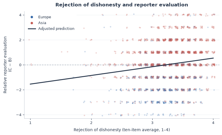
Plot rejection of dishonesty against relative reporter evaluation, with Model 5’s adjusted prediction line. Show Model 5’s adjusted country differences from Germany with 95% confidence intervals. Save both figures as PNG and PDF files in presentation_figures.
from matplotlib.lines import Line2D
import re

figure_dir = Path("presentation_figures")
figure_dir.mkdir(exist_ok=True)
blue, red, ink = "#3569A8", "#C45A53", "#253449"
report_style = {
    "font.family": "DejaVu Sans",
    "font.size": 10,
    "axes.titlesize": 12,
    "axes.titleweight": "semibold",
    "axes.labelsize": 10,
    "axes.labelpad": 8,
    "axes.edgecolor": "#BBC3CC",
    "axes.linewidth": .7,
    "text.color": ink,
    "axes.labelcolor": ink,
    "xtick.color": ink,
    "ytick.color": ink,
    "xtick.labelsize": 9,
    "ytick.labelsize": 9,
    "figure.facecolor": "white",
    "axes.facecolor": "white",
    "pdf.fonttype": 42,
    "ps.fonttype": 42,
}


def save_report_figure(fig, filename):
    # Use the PDF in Overleaf; the PNG is a high-resolution alternative.
    for extension in ["pdf", "png"]:
        path = figure_dir / f"{filename}.{extension}"
        fig.savefig(path, dpi=300, bbox_inches="tight", pad_inches=.08,
                    facecolor="white")


with plt.rc_context(report_style):
    # Figure 1: raw responses and the Model 5 adjusted prediction.
    fig, ax = plt.subplots(figsize=(7.6, 4.6), layout="constrained")
    rng = np.random.default_rng(42)
    x = analysis_5["honest_behavior"].to_numpy()
    y = analysis_5["C_minus_B"].to_numpy()
    jitter_x = x + rng.uniform(-.025, .025, len(x))
    jitter_y = y + rng.uniform(-.09, .09, len(y))
    order = rng.permutation(len(analysis_5))
    colors = np.where(analysis_5["region"].eq("Western"), blue, red)
    ax.scatter(jitter_x[order], jitter_y[order], c=colors[order],
               s=12, alpha=.25, edgecolors="none", rasterized=True, zorder=2)

    levels = np.linspace(x.min(), x.max(), 100)
    predictions = [
        model_5.predict(analysis_5.assign(honest_behavior=level)).mean()
        for level in levels
    ]
    ax.plot(levels, predictions, color=ink, linewidth=2.2, zorder=4)
    ax.axhline(0, color="#8793A1", linestyle=(0, (4, 3)), linewidth=.9, zorder=1)
    ax.set(
        title="Rejection of dishonesty and reporter evaluation",
        xlabel="Rejection of dishonesty (ten-item average, 1–4)",
        ylabel="Relative reporter evaluation\n(C − B)",
        xlim=(.9, 4.1), ylim=(-4.3, 4.3),
        xticks=[1, 2, 3, 4], yticks=[-4, -2, 0, 2, 4],
    )
    ax.set_title(ax.get_title(), loc="center", pad=12)
    ax.grid(axis="y", color="#E7EBEF", linewidth=.6)
    ax.set_axisbelow(True)
    for side in ["top", "right"]:
        ax.spines[side].set_visible(False)
    # In the Model 5 sample, the Western/Eastern groups are Europe/Asia.
    ax.legend(handles=[
        Line2D([0], [0], marker="o", color=blue, linestyle="none",
               markersize=5, label="Europe"),
        Line2D([0], [0], marker="o", color=red, linestyle="none",
               markersize=5, label="Asia"),
        Line2D([0], [0], color=ink, linewidth=2.2,
               label="Adjusted prediction"),
    ], loc="upper left", fontsize=9, frameon=True, facecolor="white",
       edgecolor="none", framealpha=.95, borderpad=.6)
    save_report_figure(fig, "honesty_associations_model5")
    plt.show()
    plt.close(fig)

    # Figure 2: Model 5 country coefficients and pointwise 95% HC3 intervals.
    country_terms = sorted(
        [term for term in model_5.params.index if term.startswith("C(cntry)")],
        key=lambda term: model_5.params[term],
    )
    fig, ax = plt.subplots(figsize=(7.6, 4.2), layout="constrained")
    row_labels = []
    for row, term in enumerate(country_terms):
        code = int(re.search(r"T\.(\d+)", term).group(1))
        beta = model_5.params[term]
        lower, upper = model_5.conf_int().loc[term]
        row_labels.append(country_labels[code])
        ax.errorbar(
            beta, row, xerr=[[beta - lower], [upper - beta]],
            fmt="o", color=blue if code in [1, 2, 9] else red,
            markersize=5.5, capsize=3.5, linewidth=1.6, zorder=3,
        )
    ax.set_yticks(range(len(row_labels)), row_labels)
    ax.set_ylim(len(row_labels) - .5, -.65)
    ax.set_title("Adjusted country differences", pad=12)
    ax.set_xlabel("Difference in relative reporter evaluation\n(reference: Germany)")
    ax.axvline(0, color="#8793A1", linestyle=(0, (4, 3)), linewidth=.9)
    ax.grid(axis="x", color="#E7EBEF", linewidth=.6)
    ax.set_axisbelow(True)
    ax.margins(x=.10)
    ax.tick_params(axis="y", length=0, pad=8)
    for side in ["top", "right", "left"]:
        ax.spines[side].set_visible(False)
    ax.legend(handles=[
        Line2D([0], [0], marker="o", color=blue, linestyle="none",
               markersize=5, label="Europe"),
        Line2D([0], [0], marker="o", color=red, linestyle="none",
               markersize=5, label="Asia"),
    ], loc="upper right", ncol=2, frameon=False, fontsize=9)
    save_report_figure(fig, "country_differences_model5")
    plt.show()
    plt.close(fig)


Regional analysis: Europe and Asia
Estimate Model 5 without country dummies separately for Europe and Asia, including power distance and individualism. Use Model 5’s eligible sample with Hong Kong pooled with China; India drops out because its index values are missing. Compare regional coefficients and confidence intervals, noting that different significance levels alone do not establish different slopes.
regional_formula = (
    "C_minus_B ~ honesty_importance + honest_behavior + age + C(gender) + C(degree) + PDI1 + IDV"
)
regional_codes = {"Europe": [1, 2], "Asia": [3, 4, 5, 6, 8]}
regional_samples = {}
regional_models = {}

for region, codes in regional_codes.items():
    sample = analysis_5.loc[analysis_5["cntry"].isin(codes)].copy()
    # Avoid empty-category coefficients after splitting the sample.
    for variable in ["gender", "degree"]:
        sample[variable] = sample[variable].cat.remove_unused_categories()
    regional_samples[region] = sample
    regional_models[region] = smf.ols(
        regional_formula, data=sample, missing="raise"
    ).fit(cov_type="HC3")
    country_counts = sample["cntry"].value_counts().sort_index()
    coverage = ", ".join(
        f"{country_labels[code]}: {int(count):,}"
        for code, count in country_counts.items() if count > 0
    )
    references = ", ".join(
        f"{variable} = {meta.variable_value_labels[variable][sample[variable].cat.categories[0]]}"
        for variable in ["gender", "degree"]
    )
    print(f"{region}: N = {len(sample):,} ({coverage})")
    print(f"Reference groups: {references}")

regional_terms = list(dict.fromkeys(
    term for model in regional_models.values() for term in model.params.index
))
regional_order = ["honesty_importance", "honest_behavior", "PDI1", "IDV", "age"] + [
    term for term in regional_terms
    if term not in ["honesty_importance", "honest_behavior", "PDI1", "IDV", "age", "Intercept"]
] + ["Intercept"]
regional_table = pd.DataFrame(index=regional_order, columns=regional_models, dtype=object)
for region, model in regional_models.items():
    for term in regional_order:
        regional_table.loc[term, region] = (
            f"{model.params[term]:.3f}{significance_mark(model.pvalues[term])} "
            f"({model.bse[term]:.3f})" if term in model.params else "—"
        )
regional_table.index = [readable_term(term) for term in regional_order]
regional_table.index.name = "Predictor / statistic"
for region, model in regional_models.items():
    regional_table.loc["Observations", region] = f"{int(model.nobs):,}"
    regional_table.loc["R²", region] = f"{model.rsquared:.3f}"
    regional_table.loc["Adjusted R²", region] = f"{model.rsquared_adj:.3f}"
    regional_table.loc["Country dummies", region] = "No"

display(
    regional_table.style
    .set_caption("Regional Model 5 regressions | beta with significance marks (HC3 standard error)")
    .set_properties(**{"text-align": "center", "padding": "9px 14px"})
    .set_table_styles([
        {"selector": "caption", "props": [("font-size", "17px"), ("font-weight", "bold"), ("text-align", "left")]},
        {"selector": "th", "props": [("text-align", "left"), ("padding", "9px 14px")]},
        {"selector": "thead th", "props": [("background-color", "#edf2f7"), ("color", "#172b4d")]},
    ])
)
print("*** p < .001; ** p < .01; * p < .05; · p < .10. All standard errors are HC3.")

regional_focus_rows = []
for region, model in regional_models.items():
    for term in ["honesty_importance", "honest_behavior"]:
        lower, upper = model.conf_int().loc[term]
        regional_focus_rows.append({
            "Sample": region,
            "Predictor": readable_term(term),
            "Beta": model.params[term],
            "HC3 SE": model.bse[term],
            "p-value": model.pvalues[term],
            "95% CI lower": lower,
            "95% CI upper": upper,
        })
regional_focus = pd.DataFrame(regional_focus_rows).set_index(["Sample", "Predictor"])
display(regional_focus.style.format({
    "Beta": "{:.3f}", "HC3 SE": "{:.3f}", "p-value": "{:.3g}",
    "95% CI lower": "{:.3f}", "95% CI upper": "{:.3f}"
}))Europe: N = 626 (Germany: 569, Estonia: 57) Reference groups: gender = Male, degree = High school Asia: N = 1,591 (Taiwan: 611, China (incl. Hong Kong): 524, Vietnam: 340, Japan: 116) Reference groups: gender = Male, degree = High school
| Europe | Asia | |
|---|---|---|
| Predictor / statistic | ||
| Honesty importance | -0.014 (0.061) | 0.062· (0.036) |
| Rejection of dishonesty | 0.532** (0.195) | 0.652*** (0.098) |
| Power distance (PDI1) | 0.000 (0.001) | 0.000 (0.001) |
| Individualism (IDV) | -0.008*** (0.002) | -0.001 (0.001) |
| Age (years) | -0.006 (0.014) | 0.006 (0.007) |
| Gender: Female | 0.039 (0.130) | 0.063 (0.081) |
| Gender: others | 1.313 (1.302) | -0.054 (0.662) |
| Education: Bachelor | 0.102 (0.147) | 0.040 (0.102) |
| Education: Master | 0.921*** (0.274) | 0.239· (0.133) |
| Education: PhD | -0.543 (0.575) | -0.147 (0.340) |
| Education: Other | -0.349 (0.808) | -0.075 (0.202) |
| Intercept | -2.252** (0.756) | -2.006*** (0.379) |
| Observations | 626 | 1,591 |
| R² | 0.104 | 0.044 |
| Adjusted R² | 0.088 | 0.038 |
| Country dummies | No | No |
*** p < .001; ** p < .01; * p < .05; · p < .10. All standard errors are HC3.
| Beta | HC3 SE | p-value | 95% CI lower | 95% CI upper | ||
|---|---|---|---|---|---|---|
| Sample | Predictor | |||||
| Europe | Honesty importance | -0.014 | 0.061 | 0.82 | -0.134 | 0.106 |
| Rejection of dishonesty | 0.532 | 0.195 | 0.00627 | 0.150 | 0.913 | |
| Asia | Honesty importance | 0.062 | 0.036 | 0.0818 | -0.008 | 0.132 |
| Rejection of dishonesty | 0.652 | 0.098 | 2.3e-11 | 0.461 | 0.843 |
Project report
Read the full report here, or open the PDF in a separate tab.